Adapting the photon sampling

In my previous implementations of the occlusion map, occlusion photons were created at every intersection point along an occlusion ray. However, this approach has a few downsides when we are generating the occlusion rays from the camera or uniform in the scene. For uniform sampling, we are breaking uniform distribution of the occlusion photons. For camera sampling, we are creating occlusion photons at positions which are not visible from the camera. Therefore, I have rewritten the photon sampling methods so that I am able to disable the recursive occlusion photon creation. (please note that the recursive photon creation is still necessary when sampling the light sources, otherwise the photons might not be distributed in the visible locations of the scene)

The following image illustrates how removing the recursion distributes the photons better in the visible locations of the scene when using camera sampling:

Figure 1: Camera sampling with and without the recursion

The following images show some rendered images with the new modified sampling techniques:

Light sampling 200K photons	Light sampling: photon density 200K photons
Uniform sampling 200K photons	Uniform sampling: photon density 200K photons
Camera sampling 200K photons	Camera sampling: photon density 200K photons

The left images show the results rendered with the occlusion map at 200K photons without the use of volumetric occluders. The images on the right show a plot of the density of the occlusion photons where black pixels contain no occlusion photons and bright spots contain a lot of photons.

When we use light sampling, we can see that the density of the occlusion photons drops as the distance from the light source increases, which is what we expect. This is most noticable when we compare the shadows of the killeroos.

Uniform sampling succeeds in distributing the photons more evenly. This is also most noticable in the shadows of the killeroos. The distribution does not seem very uniform on the killeroo's themselves but this is expected as not every position on the killeroo can generate an occlusion photon.

Note that for the photon plot I positioned the camera a little more backwards to highlight the fact that no  occlusion photons are stored at invisible locations of the scene. That's why the photon density plot of the camera sampling technique cuts of the shadow of the right killeroo. As the photon density plot clearly show, the occlusion photon locations exactly match the shadowed regions onthe killeroo.

Conclusion

From the resulting images, camera sampling is clearly the best option in terms of quality, because it places the occlusion photons in the most relevant positions of the scene. The downside of camera sampling is that we have to rebuild the occlusion map when the camera is moved. For interactive applications, uniform sampling would be a better choice, however, it takes the longest to compute. This is because we use a global line sampling (which misses a lot of the geometry) to generate uniform occlusion photons locations. This was necessary since, PBRT doesn't allow you to directly access the geometry of the scene.

Creating the volumetric occluders

In my previous blog post I implemented a first version of occlusion mapping. There were still a couple of problems with the approach, which I will recapitulate in the first section. I also proposed the usage of "Volumetric occluders" as partial solution to some of these problems. How these occluders are constructed and pseudo code of the implementation will be given in the second section. I will conclude with some resulting pictures.

Problems with occlusion mapping

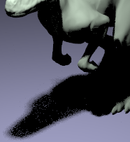
The main problem of occlusion mapping are light points in shadow regions (see figure 1). These light points occur when not all of the geometry is represented in the occlusion map. This can occur in a couple of situations:

• not enough occlusion photons are shot
• some (small) primitives in the model are not hit by any occlusion rays

The first situation is obvious. Imagine an exagerated example in which we have a model with 1000 triangles, while the occlusion map only contains 100 occluders. This means that 900 triangles will never be intersected for shadows.

The second situation occurs when the directions from which occlusion rays are shot are chosen in a unfortunate way, thereby missing some triangles. From the last blog post, we could see that shooting occlusion rays to the visible parts of the scene certainly helped, however it could not resolve the problem completely.

Therefore I suggested to create volumetric occluders inside the model. While small triangles in the model can be missed, it is less likely that large occluders inside the model are missed. In the following section I will discuss how the volumetric occluders can be created.

Figure 1: Light points in the shadow region.

Creating volumetric occluders

I got the idea of using volumetric occluder from the paper "Accelerating Shadow Rays Using Volumetric Occluders and Modified kd-Tree Traversal" (2009) by Peter Djeu, Sean Keely, and Warren Hunt.

They created a kd-tree over a watertight and manifold model. They use a modified version of the surface area heuristic which favors empty leaf nodes in the kd-tree. When the kd-tree is finished, the leaf nodes are marked to be either:

• opaque: it is inside the model
• boundary: it contains geometry of the model
• clear: the node is located outside the model

Labeling boundary nodes is straightforward. We only need to check whether the node contains geometry. If it contains geometry, it is a boundary node.

Labelling a leaf node as clear or opaque is done by casting a ray in a random direction from anywhere within the leaf node. They made the observation that when a ray originates from inside the model, it always has to intersect the model. Furtermore, the normal should be in the same direction as the direction of the ray (their dot product should always be positive).

If the ray misses the geometry of the model or hits a front-facing primitive of the model, we know it is located outside the model and the leaf node is marked as clear. If the ray hits a back-facing primitive of the model, we know it has to be located inside the model and the leaf node is marked opaque. 

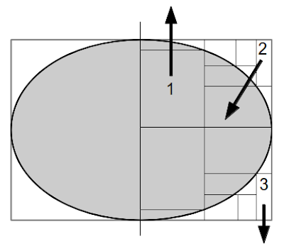
The labelling process is illustrated in the figure 2. The ellips represents some geometry bounded by a rectanglular gray box. The black lines represent kd splitting planes. The node labelled 1, will be marked as an opaque node since the ray (black arrow) hits the geometry from the back side. Node 2 will be marked as clear, since it intersects the geometry from the front side. Node 3 will also be labelled as clear, since it misses all the geometry (which would be impossible if the ray was shot from inside the model).

Figure 2: The marking process of the nodes. Node 1 is opaque since it hits the back of the geometry.
Node 2 is clear since it hits the geometry from up front. Node 3 is clear since it does not
intersect any geometry.

However, I chose to construct an octree over the model instead of a kd-tree. This makes it alot easier to extract the volumetric occluders. With kd-trees we first need to determine which planes bound a leaf node and construct the volumetric occluder from the intersections of the bounding planes. With an octree we can just use the subdivisions of the bounding box.

The pseudocode for the construction is given below.


vector<BBox> occluders;
Mesh model;

vector<BBox> recursiveBuild(primitivesInBoundingBox, boundingBox, depth) {
    // Divide the bounding box in 8 sub boxes.
    vector<BBox> subBoxes = subdivide(boundingbox);
    vector<Primitive> primsInSubBox[8];

    // Place the primitives in the correct sub box
    for(int i=0;i<subBoxes.size(); ++i)
      for(primitive in primitivesInBoundingBox
        if (primitive.WorldBound().overlaps(subBoxes[i])
          primsInSubBox[i].push_back(primitive);

    // Label the empty nodes as opaque or clear
    for(int i=0;i<subBoxes.size(); ++i)
      if (primsInSubBox[i].size() == 0) {
        Point origin = subBoxes[i].center;
        Vector direction = generateRandomDirection();
        Ray ray(center,direction);
        Intersection isect;
        if (model->Intersect(ray,&isect)
          if (direction.dot(isect.normal) > 0) {
            occluders.push_back(subBoxes[i]);
            break;
          }
      }

    // Apply recursion
    if (depth > 0)
      for(int i=0;i<subBoxes.size();++i)
        if (primsInSubBox[i].size() > 0)
          recursiveBuild(primsInSubBox[i],subBox[i],depth-1);
}

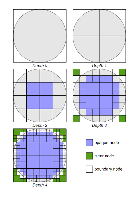
This algorithm is shown in progress for different depth levels in the figure below:

Figure 3: Octree subdivision

Results

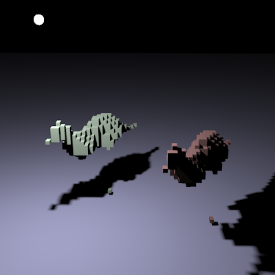
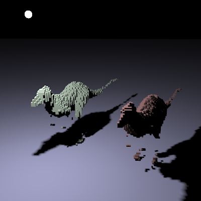
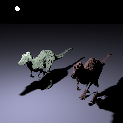
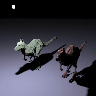
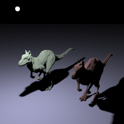
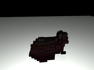
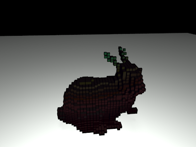
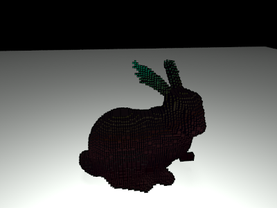
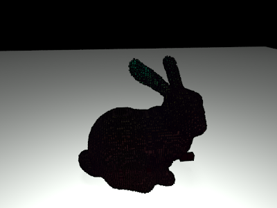
The figures below show the algorithm implemented in PBRT for the killeroo and bunny scene and different maximum recursion depths:

Killeroo-scene

Figure 4: Occluder creation with maximum recursion depth 4

Figure 5: Occluder creation with maximum recursion depth 5

Figure 6: Occluder creation with maximum recursion depth 6

Figure 7: Occluder creation with maximum recursion depth 7

Figure 8: Occluder creation with maximum recursion depth 8

Bunny scene

Figure 9: Occluder creation with maximum recursion depth 3

Figure 10: Occluder creation with maximum recursion depth 4

Figure 11: Occluder creation with maximum recursion depth 5

Figure 12: Occluder creation with maximum recursion depth 6

Conclusion

The algorithm is implemented, however, it only works correctly for the killeroo scene at the moment. This is the only scene in which the model is stored as one complete mesh (e.g. the teapot is a combination of a lot of seperate shapes) that is watertight and manifold. The bunny is partially correct, however, there are some errors in the occluders (I'm not sure why yet).

The number of occluders can become large at higher recursion depths. However, it could be possible to combine multiple occluders to one larger occluder. This would decrease storage requirements by a large amount and increase performance.

The next step is combining the occluders with the occlusion mapping technique. When this is done and gives good results, probabilistic visibility will be added to make clever occluder selections.