Paper - First Draft

I finished my first draft of my paper. The paper can be downloaded from this link Probablistic Visibility with the Occlusion Map. I will kindly return the favor to students who would like to review my paper ;)

Thesis utilities

For my thesis, I created some tools to help me along the way. I made the source code to these tools publicly available at github. I can only encourage other people to use and improve these tools.

Random scene generator

The first tool is a random scene generator.  This Java program allows you to create a cornell box in which user-specified model is inserted a random locations.The following image shows the result of a scene with 343 icosahedrons. To create the scene, it is divided into equal sized voxels and in each voxel an icosahedron is placed. This avoid cluming of the geometry into one location.

The code is available at: https://github.com/NielsBillen/PBRTRandomSceneGenerator

Figure 1: Random cornell box with 343 icosahedrons

Batch rendering tool

The following tool allows you to render a batch of scenes. The program uses a stripped down scene file as input, inserts your specific parameters into the scene file (e.g. Surfaceintegrator "directlighting" "string strategy" ["one"]) and executes it. 

It is also possible to distribute jobs over multiple pc's using SSH. 

The code is available at: https://github.com/NielsBillen/PBRTBatchRendering

Adapting the photon sampling

In my previous implementations of the occlusion map, occlusion photons were created at every intersection point along an occlusion ray. However, this approach has a few downsides when we are generating the occlusion rays from the camera or uniform in the scene. For uniform sampling, we are breaking uniform distribution of the occlusion photons. For camera sampling, we are creating occlusion photons at positions which are not visible from the camera. Therefore, I have rewritten the photon sampling methods so that I am able to disable the recursive occlusion photon creation. (please note that the recursive photon creation is still necessary when sampling the light sources, otherwise the photons might not be distributed in the visible locations of the scene)

The following image illustrates how removing the recursion distributes the photons better in the visible locations of the scene when using camera sampling:

Figure 1: Camera sampling with and without the recursion

The following images show some rendered images with the new modified sampling techniques:

Light sampling 200K photons	Light sampling: photon density 200K photons
Uniform sampling 200K photons	Uniform sampling: photon density 200K photons
Camera sampling 200K photons	Camera sampling: photon density 200K photons

The left images show the results rendered with the occlusion map at 200K photons without the use of volumetric occluders. The images on the right show a plot of the density of the occlusion photons where black pixels contain no occlusion photons and bright spots contain a lot of photons.

When we use light sampling, we can see that the density of the occlusion photons drops as the distance from the light source increases, which is what we expect. This is most noticable when we compare the shadows of the killeroos.

Uniform sampling succeeds in distributing the photons more evenly. This is also most noticable in the shadows of the killeroos. The distribution does not seem very uniform on the killeroo's themselves but this is expected as not every position on the killeroo can generate an occlusion photon.

Note that for the photon plot I positioned the camera a little more backwards to highlight the fact that no  occlusion photons are stored at invisible locations of the scene. That's why the photon density plot of the camera sampling technique cuts of the shadow of the right killeroo. As the photon density plot clearly show, the occlusion photon locations exactly match the shadowed regions onthe killeroo.

Conclusion

From the resulting images, camera sampling is clearly the best option in terms of quality, because it places the occlusion photons in the most relevant positions of the scene. The downside of camera sampling is that we have to rebuild the occlusion map when the camera is moved. For interactive applications, uniform sampling would be a better choice, however, it takes the longest to compute. This is because we use a global line sampling (which misses a lot of the geometry) to generate uniform occlusion photons locations. This was necessary since, PBRT doesn't allow you to directly access the geometry of the scene.

Creating the volumetric occluders

In my previous blog post I implemented a first version of occlusion mapping. There were still a couple of problems with the approach, which I will recapitulate in the first section. I also proposed the usage of "Volumetric occluders" as partial solution to some of these problems. How these occluders are constructed and pseudo code of the implementation will be given in the second section. I will conclude with some resulting pictures.

Problems with occlusion mapping

The main problem of occlusion mapping are light points in shadow regions (see figure 1). These light points occur when not all of the geometry is represented in the occlusion map. This can occur in a couple of situations:

• not enough occlusion photons are shot
• some (small) primitives in the model are not hit by any occlusion rays

The first situation is obvious. Imagine an exagerated example in which we have a model with 1000 triangles, while the occlusion map only contains 100 occluders. This means that 900 triangles will never be intersected for shadows.

The second situation occurs when the directions from which occlusion rays are shot are chosen in a unfortunate way, thereby missing some triangles. From the last blog post, we could see that shooting occlusion rays to the visible parts of the scene certainly helped, however it could not resolve the problem completely.

Therefore I suggested to create volumetric occluders inside the model. While small triangles in the model can be missed, it is less likely that large occluders inside the model are missed. In the following section I will discuss how the volumetric occluders can be created.

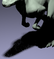Figure 1: Light points in the shadow region.

Creating volumetric occluders

I got the idea of using volumetric occluder from the paper "Accelerating Shadow Rays Using Volumetric Occluders and Modified kd-Tree Traversal" (2009) by Peter Djeu, Sean Keely, and Warren Hunt.

They created a kd-tree over a watertight and manifold model. They use a modified version of the surface area heuristic which favors empty leaf nodes in the kd-tree. When the kd-tree is finished, the leaf nodes are marked to be either:

• opaque: it is inside the model
• boundary: it contains geometry of the model
• clear: the node is located outside the model

Labeling boundary nodes is straightforward. We only need to check whether the node contains geometry. If it contains geometry, it is a boundary node.

Labelling a leaf node as clear or opaque is done by casting a ray in a random direction from anywhere within the leaf node. They made the observation that when a ray originates from inside the model, it always has to intersect the model. Furtermore, the normal should be in the same direction as the direction of the ray (their dot product should always be positive).

If the ray misses the geometry of the model or hits a front-facing primitive of the model, we know it is located outside the model and the leaf node is marked as clear. If the ray hits a back-facing primitive of the model, we know it has to be located inside the model and the leaf node is marked opaque. 

The labelling process is illustrated in the figure 2. The ellips represents some geometry bounded by a rectanglular gray box. The black lines represent kd splitting planes. The node labelled 1, will be marked as an opaque node since the ray (black arrow) hits the geometry from the back side. Node 2 will be marked as clear, since it intersects the geometry from the front side. Node 3 will also be labelled as clear, since it misses all the geometry (which would be impossible if the ray was shot from inside the model).

Figure 2: The marking process of the nodes. Node 1 is opaque since it hits the back of the geometry.
Node 2 is clear since it hits the geometry from up front. Node 3 is clear since it does not
intersect any geometry.

However, I chose to construct an octree over the model instead of a kd-tree. This makes it alot easier to extract the volumetric occluders. With kd-trees we first need to determine which planes bound a leaf node and construct the volumetric occluder from the intersections of the bounding planes. With an octree we can just use the subdivisions of the bounding box.

The pseudocode for the construction is given below.


vector<BBox> occluders;
Mesh model;

vector<BBox> recursiveBuild(primitivesInBoundingBox, boundingBox, depth) {
    // Divide the bounding box in 8 sub boxes.
    vector<BBox> subBoxes = subdivide(boundingbox);
    vector<Primitive> primsInSubBox[8];

    // Place the primitives in the correct sub box
    for(int i=0;i<subBoxes.size(); ++i)
      for(primitive in primitivesInBoundingBox
        if (primitive.WorldBound().overlaps(subBoxes[i])
          primsInSubBox[i].push_back(primitive);

    // Label the empty nodes as opaque or clear
    for(int i=0;i<subBoxes.size(); ++i)
      if (primsInSubBox[i].size() == 0) {
        Point origin = subBoxes[i].center;
        Vector direction = generateRandomDirection();
        Ray ray(center,direction);
        Intersection isect;
        if (model->Intersect(ray,&isect)
          if (direction.dot(isect.normal) > 0) {
            occluders.push_back(subBoxes[i]);
            break;
          }
      }

    // Apply recursion
    if (depth > 0)
      for(int i=0;i<subBoxes.size();++i)
        if (primsInSubBox[i].size() > 0)
          recursiveBuild(primsInSubBox[i],subBox[i],depth-1);
}

This algorithm is shown in progress for different depth levels in the figure below:

Figure 3: Octree subdivision

Results

The figures below show the algorithm implemented in PBRT for the killeroo and bunny scene and different maximum recursion depths:

Killeroo-scene

Figure 4: Occluder creation with maximum recursion depth 4

Figure 5: Occluder creation with maximum recursion depth 5

Figure 6: Occluder creation with maximum recursion depth 6

Figure 7: Occluder creation with maximum recursion depth 7

Figure 8: Occluder creation with maximum recursion depth 8

Bunny scene

Figure 9: Occluder creation with maximum recursion depth 3

Figure 10: Occluder creation with maximum recursion depth 4

Figure 11: Occluder creation with maximum recursion depth 5

Figure 12: Occluder creation with maximum recursion depth 6

Conclusion

The algorithm is implemented, however, it only works correctly for the killeroo scene at the moment. This is the only scene in which the model is stored as one complete mesh (e.g. the teapot is a combination of a lot of seperate shapes) that is watertight and manifold. The bunny is partially correct, however, there are some errors in the occluders (I'm not sure why yet).

The number of occluders can become large at higher recursion depths. However, it could be possible to combine multiple occluders to one larger occluder. This would decrease storage requirements by a large amount and increase performance.

The next step is combining the occluders with the occlusion mapping technique. When this is done and gives good results, probabilistic visibility will be added to make clever occluder selections.

Occlusion Mapping - First Implementation

I've started on the implementation of occlusion mapping in PBRT. Adding a new shader is quite easy in PBRT. You only need to add another class that extends the SurfaceIntegrator class. Since my approach is similar to photon mapping, I could reuse a lot of code from the photon mapping class.

In my implementation, I programmed three rendering techniques and three techniques to distribute the occlusion photons through the scene. In the following sections, I'll discuss their implementation and their impact on the rendered images.

Terminology

I'd like to start by going through the terminology that I will use in this (and future) blog posts:

• Occlusion map: a kd-tree which stores light and occlusion photons for a specific light source.
• Light photon: a photon that indicates that a position in the scene is visible by a light source.
• Occlusion photon: a photon that indicates that a position is occluded. It also stores a list with all the occluders of that position.
• Occlusion ray: a ray which is traced through the scene and creates the light and occlusion photons. Depending on the technique, it will create a light photon upon it's first intersection. On the subsequent intersections, occlusion photons will be created.

Implementation

I described two different approaches to occlusion mapping, as described in the previous blog post on Occlusion Mapping; one with light photons and one without light photons. I implemented both of them.

Furthermore, I added one more approach in the implementation which I got from the paper "Efficiently rendering shadows using the photon map" by Henrik Wann Jensen et al. In this paper they approximate the visibility by using the ratio of light photons versus light plus shadow photons.

visibility = #light photons / (#light photons + #shadow photons)

The occlusion photons can be distributed in a different number of ways through the scene. I implemented three ways for generating the occlusion photons: from the light source, from the camera and uniform over the surfaces.

Occlusion rays from the light source

Occlusion rays are traced through the scene a light sources and a halton sequence is used to determine a random position and direction for the occlusion ray. The light source is selected using a cumulative distribution function based on the power of the light sources (stronger lights receive more photons). On each intersection excluding the first, an occlusion photon is generated. Figure 1 displays this approach:

Figure 1: Light source sampling. Occlusion rays (striped lines) are shot from the light source.
Upon each intersection, except for the first intersection, an occlusion photon is stored.

Occlusion rays from the camera

Camera rays are traced randomly from the camera's viewpoint. The first intersection point of this ray will be used to determine the direction to shoot occlusion rays to. The origin of the occlusion ray is determined by selecting a random point on a light source. The light source is selected by the cumulative distribution function of the power of the light sources. This technique is displayed in figure 2:

Figure 2: Camera sampling. First camera rays (blue lines) are traced from the camera. Their
first intersection points are used to determine the direction of the occlusion rays (red lines).
The origin of the occlusion rays is determined by taking a point on a light source using
a cummulative distribution function. 

Uniform occlusion rays

With this technique we want the density of the occlusion photons to be evenly distributed through the scene. To accomplish this, I used global line sampling (since PBRT does not allow you to acces the geometry of the scene directly). With this technique, random rays are shot through the scene and each surface has a chance proportional to it's surface area to be hit.

First the bounding sphere of the scene is determined. Then two points are randomly generated on this sphere and a ray connecting these two points is shot through the scene.

One of the intersection points of these rays is randomly selected, and chosen to be the direction to shoot the occlusion rays to. The origin of the occlusion rays is determined as described in the previous subsection; by choosing a random point on a light source. 

This technique is shown in figure 3:

Figure 3: Uniform sampling. Random rays (red lines) are shot through the scene. One of their intersection
points is chosen and used as the direction to shoot occlusion rays (blue lines) to. The origin of the
occlusion rays is determined by choosing a random point on the light source.

Results

The images below show some of the results along with the used parameters and rendering times. All of the scenes were rendered on the following hardware: Intel Core i7 - 2630QM at 2.0 Ghz, 6GB of DDR3 running Ubuntu 12.04 (64-bit).

Comparison of the rendering techniques

First I will compare the different techniques (occlusion mapping without light photons, occlusion mapping with light photons and the technique by Jensen) with each other. The results below are rendered with the three techniques and compared to a standard ray-traced image. The images show the killeroo scene that comes with PBRT, with 8 samples per pixel.

Rendering with 10,000 photons (light source radius 1)

Occlusion mapping without light photons. Number of photons: 11903 Average number of occluders per photon: 1.90817 Occlusion shooting time: 0.118894s Rendering time: 2.64184s Total time: 2.76073s	Occlusion mapping with light photons. Number of photons: 25912 Average number of occluders per photon: 0.231283 Occlusion shooting time: 0.094949s Rendering time: 2.63185s Total time: 2.7268s
Jensen's technique. Number of photons: 25925 Average number of occluders per photon: 0.231514 Occlusion shooting time: 0.107828 Rendering time: 2.57188s Total time: 2.67971s	Direct lighting. Total time: 14.2238s

Rendering with 100,000 photons (light source radius 1)

Occlusion mapping without light photons. Number of photons: 101844 Average number of occluders per photon: 1.89236 Occlusion shooting time: 0.768156s Rendering time: 3.19457s Total time: 3.96273s	Occlusion mapping with light photons. Number of photons: 115409 Average number of occluders per photon: 0.225866 Occlusion shooting time: 0.188688s Rendering time: 3.19719s Total time: 3.38588s
Jensen's technique. Number of photons: 115350 Average number of occluders per photon: 0.225626 Occlusion shooting time: 0.184848s Rendering time: 2.87288s Total time: 3.05773s	Direct lighting. Total time: 14.2238s

Rendering with 1,000,000 photons (light source radius 1)

Occlusion mapping without light photons. Number of photons: 1001683 Average number of occluders per photon: 1.8944 Occlusion shooting time: 8.53205s Rendering time: 6.40291s Total time: 14.9935s	Occlusion mapping with light photons. Number of photons: 1015612 Average number of occluders per photon: 0.225866 Occlusion shooting time: 1.96708s Rendering time: 6.92928s Total time: 8.89636s
Jensen's technique. Number of photons: 115350 Average number of occluders per photon: 0.225626 Occlusion shooting time: 1.95626s Rendering time: 5.60054s Total time: 7.55659s	Direct lighting. Total time: 14.2238s

Rendering with 100,000 photons (light source radius 3)

Occlusion mapping without light photons. Number of photons: 101675 Average number of occluders per photon: 1.89546 Occlusion shooting time: 0.786429s Rendering time: 3.45047s Total time: 4.2369s	Occlusion mapping with light photons. Number of photons: 115387 Average number of occluders per photon: 0.227209 Occlusion shooting time: 0.187175s Rendering time: 3.13611s Total time: 3.32329s
Jensen's technique. Number of photons: 115346 Average number of occluders per photon: 0.2269 Occlusion shooting time: 0.18869s Rendering time: 2.96835s Total time: 3.15704s	Direct lighting. Total time: 14.6854s

Rendering with 1,000,000 photons (light source radius 3)

Occlusion mapping without light photons. Number of photons: 1001686 Average number of occluders per photon: 1.89493 Occlusion shooting time: 8.58199s Rendering time: 6.75203s Total time: 15.334s	Occlusion mapping with light photons. Number of photons: 115387 Average number of occluders per photon: 0.227209 Occlusion shooting time: 1.9558s Rendering time: 7.1825s Total time: 9.1383s
Jensen's technique. Number of photons: 1014080 Average number of occluders per photon: 0.225214 Occlusion shooting time: 2.02617s Rendering time: 5.78872s Total time: 7.81489s	Direct lighting. Total time: 14.6854s

The above sequence of images shows that for a large number of occlusion photons the results converges to the correct image. Furthermore we can make the following remarks about the three techniques:

1. Occlusion mapping without light photons is best at preserving the shadow boundaries. The difficulty with this technique is that when a small number of occlusion photons is created, light dots are formed inside the shadow (will be discussed further)
2. Occlusion mapping with light photons partially solves this problem. Thanks to the light photons, shadow rays will only be traced in the penumbra regions (the soft shadow regions), because light photons will never occur in regions which are fully in shadow. The problem with this technique is that there is less information about the occluders in the occlusion map (the average number of occluders per photons is only around 0.2 per photon).
3. Jenssens technique is only added for comparing the other two techniques with a technique that does not trace any shadow rays. The ratio of light photons versus light and occlusion photons is only a rough estimate. To get exact results a prohibitive number of photons would need to be stored and the lookup radius for the occlusion map should nearly be zero.

Comparison of the occlusion shooting methods

Finally we compare the methods for distributing the occlusion photon in the scene. For this we render the killeroo scene with 100,000 and 1,000,000 occlusion photons (no light photons).

Rendering with 100,000 occlusion photons

Light sampling
Average number of occluders per occlusion photon: 1.89528
Occlusion photon shooting time: 0.863877s
Render time: 3.36405s
Total time: 4.22793s

Camera sampling
Average number of occluders per occlusion photon: 2,14348
Occlusion photon shooting time: 0.504893s
Render time: 3.96897s
Total time: 4,47387s

Uniform sampling
Average number of occluders per occlusion photon: 1,87973
Occlusion photon shooting time: 25.7469s
Render time: 3.40524s
Total time: 29.1521s

Rendering with 1,000,000 occlusion photons

Light sampling
Average number of occluders per occlusion photon: 1,87973
Occlusion photon shooting time: 8,52909s
Render time: 6,69704s
Total time: 15,2261s

Camera sampling
Average number of occluders per occlusion photon: 2,14517
Occlusion photon shooting time: 3,59355s
Render time: 6,98851s
Total time: 10,5821s

Uniform sampling
Average number of occluders per occlusion photon: 1,87756
Occlusion photon shooting time: 298,16s
Render time: 6,97551
Total time: 305,135s

From the resulting images we can conclude that camera sampling is the most effective way. On average, more occlusion information is stored. Thanks to the camera driven construction of the occlusion map, we can be certain that occlusion photons are stored in visible locations. Finally we can see that the resulting images are better (compare the right flank of the right killeroo in the images).

Camera sampling is also more efficient in the time needed to construct the occlusion map. Light sampling wastes a lot of time shooting rays in directions that do not have any geometry. The global line sampling algorithm for uniform sampling also generates a lot of rays that do not intersect any geometry in the scene.

Conclusion

The current implementation still has some issues. The main issue that occurs are the light spots in the shadow regions, which can be seen in the figure below:

Light spots in the shadow regions

These light spots occur because some triangles in the mesh are never hit by any occlusion ray. This means that these triangles can never be tested for occlusion leading to false misses during rendering. This problem will become even more severe when the light sources are large.

A solution to this problem would be to create large volumetric occluders inside the models and to store these volumetric occluders inside the occlusion photons too. This will partially resolve the problem because altough occlusion rays may miss some small triangles, they are less likely to miss the larger volumetric occluders. The volumetric occluders can also be used to increase the performance. Since it is more likely that a volumetric occluder is hit than that a triangle of the mesh is hit (since volumetric occluders are usually large), we can choose to intersect the volumetric occluders first (which are cheaper to intersect).

Occlusion mapping with light photons also solves the problem of the light spots in the shadow regions.

No shadow rays will be shot from regions that are in full shadow because they can't contain any light photons. Therefore the false misses are avoided. The downside is that when light photons are used, less information about occlusion is stored in the occlusion map for the same number of photons. (without light photons, the average number of occluders per photon is 1.8; with light photons, the average number of occluders per photon is 0.2)

Finally, we could also store neighbouring triangles of an occluder in an occlusion photon. This could affect performance, since the number of stored occluders will increase by a great amount.